

A decision tree is the most honest model in machine learning. It is a flowchart: ask a yes/no question about one column, follow the branch, ask another question, and stop when you reach an answer. The only clever part is that the computer picks the questions for you.
In this article we build one on a real medical problem, the Pima Indians Diabetes dataset, and use it to learn the core ideas of supervised learning: splitting data, choosing metrics, reading a model, and catching it when it memorises instead of learns.
The data: 768 patients, one question#
Each row is a woman of Pima heritage aged 21 or older, described by eight clinical measurements: number of pregnancies, plasma glucose, blood pressure, skin-fold thickness, insulin, BMI, a diabetes pedigree score (family history) and age. The target, Outcome, is 1 if she was diagnosed with diabetes and 0 otherwise.
import pandas as pd

df = pd.read_csv("diabetes.csv")
df.shape                                   # (768, 9)
df["Outcome"].value_counts(normalize=True) # 0: 0.651, 1: 0.349
Two things to notice before touching a model.
The classes are unequal. About 65% of patients are non-diabetic. A model that always answers "no diabetes" would score 65% accuracy while being useless. Keep that number in mind; it is the floor every real model has to beat.
isnull() lies here. Run df.isnull().sum() and you get zeros everywhere, which looks clean. But 374 patients have an insulin reading of 0, 227 have a skin thickness of 0, and 11 have a BMI of 0. Nobody alive has a BMI of zero. Those are missing values wearing a disguise. Trees are fairly robust to this (a zero just lands on one side of a split), but for many other models you would need to treat these as missing. Always look at the minimums in df.describe().
How a tree picks its questions#
Before the first split, the whole training set sits in one node: 65% "no", 35% "yes". The tree needs a number for how mixed that node is. The usual choice is Gini impurity:
Gini = 1 - (p_no² + p_yes²)
     = 1 - (0.651² + 0.349²)
     = 0.454
A node containing only one class has Gini 0 (perfectly pure). A 50/50 node has Gini 0.5, the worst possible for two classes. Think of it as the chance that two patients picked at random from the node have different labels.
To grow the tree, the algorithm tries every column and every threshold, splits the data in two, and computes the weighted Gini of the two children. It keeps whichever split lowers impurity the most, then repeats inside each child. That is the entire algorithm. It is greedy (it never looks ahead) and it is fast.
You can often predict the first split just by looking at the data. Plot glucose for each group:
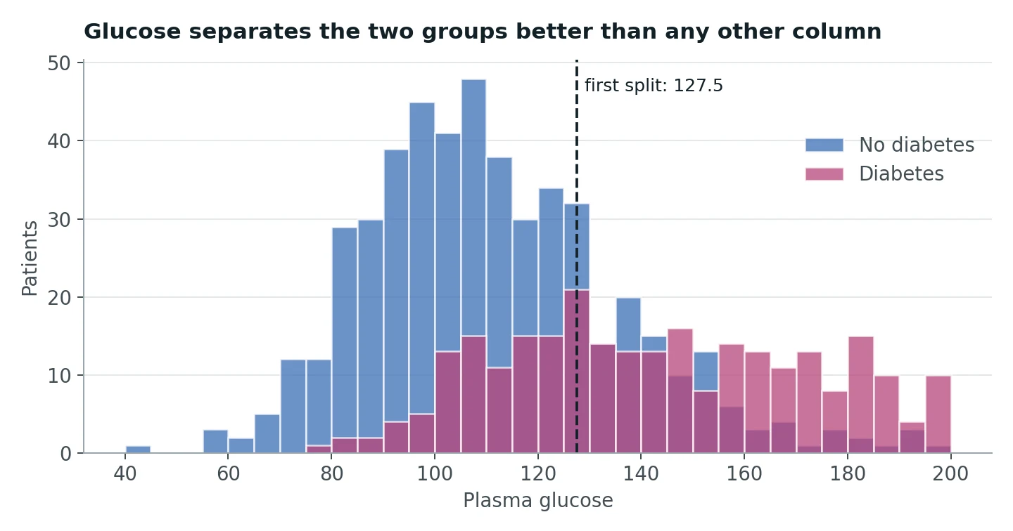
The non-diabetic patients cluster around 100 to 110, the diabetic patients spread to the right. Glucose has the strongest correlation with the outcome (0.47, against 0.29 for BMI, the next best), and sure enough, the tree's very first question is Glucose <= 127.5.
Training, with the golden rule#
The golden rule of evaluation: never grade a model on data it trained on. That is like studying from the answer key and calling it an exam. We hold back 20% of patients, and stratify=y keeps the 65/35 ratio identical in both halves.
from sklearn.model_selection import train_test_split
from sklearn.tree import DecisionTreeClassifier

X = df.drop(columns="Outcome")
y = df["Outcome"]
X_train, X_test, y_train, y_test = train_test_split(
    X, y, test_size=0.20, random_state=42, stratify=y
)

clf = DecisionTreeClassifier(
    max_depth=5,             # at most 5 questions per path
    min_samples_leaf=5,      # no leaf smaller than 5 patients
    min_samples_split=10,
    class_weight="balanced", # make the minority class count as much as the majority
    random_state=42,
).fit(X_train, y_train)
class_weight="balanced" upweights the diabetic patients so the tree cannot win by ignoring them. One side effect: the root node now reports Gini 0.5, because after reweighting the two classes count equally.
Accuracy is not the whole story#
This tree scores 80.0% on training data and 75.3% on the test set. Good, but the confusion matrix tells us what kind of mistakes it makes:
| Predicted no | Predicted yes | |
|---|---|---|
| Actually no (100) | 72 | 28 |
| Actually yes (54) | 10 | 44 |
Now the four numbers everyone should be able to derive from that table:
- Recall for diabetes = 44 / 54 = 0.815. Of the patients who really had diabetes, we caught 81%.
- Precision for diabetes = 44 / 72 = 0.611. Of the patients we flagged, 61% really had it.
- F1 combines the two (their harmonic mean): 0.698.
- Recall for the non-diabetic class is only 0.72: 28 healthy patients were flagged.
Which matters more depends on what the model is for. As a screening tool, a missed diabetic (false negative) goes home untreated, while a false alarm gets a follow-up blood test. For screening you would happily trade some precision for recall. Accuracy hides that trade entirely.
One split is one opinion; cross-validation is a panel#
A single 80/20 split depends on which 154 patients happened to land in the test set. Five-fold cross-validation trains five trees, each tested on a different fifth of the data:
from sklearn.model_selection import StratifiedKFold, cross_val_score

cv = StratifiedKFold(n_splits=5, shuffle=True, random_state=42)
scores = cross_val_score(clf, X, y, cv=cv)
# [0.760, 0.753, 0.643, 0.699, 0.634]  mean 0.698 ± 0.053
The fold scores range from 63% to 76%. Our 75.3% test score was a lucky draw; 69.8% is the more honest estimate. Individual trees are high-variance models: small changes in the data produce noticeably different trees. (That weakness is exactly what random forests fix, which is a story for another article.)
Reading the model#
This is the part no neural network can offer. Feature importance tells us how much each column reduced impurity across the whole tree:
| Feature | Importance |
|---|---|
| Glucose | 0.529 |
| BMI | 0.208 |
| Age | 0.125 |
| Diabetes pedigree | 0.090 |
| Insulin, pregnancies, blood pressure | under 0.03 each |
| Skin thickness | 0.000 |
Skin thickness has zero importance, meaning the tree never used it. That does not prove it is useless medically; it means that once glucose, BMI and age were known, it added nothing this tree could use (and remember, 227 of its values were fake zeros).
export_text prints the tree as rules. One path through it reads:
IF glucose > 127.5 AND BMI > 29.95 AND glucose > 157.5 THEN predict diabetes.
A clinician can check that against their own experience in seconds. That is the superpower of trees.
Watching a tree overfit#
What happens if we let the tree grow deeper? I trained trees of depth 1 to 20 and tracked training accuracy against cross-validated accuracy:
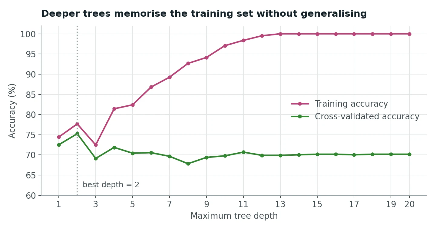
This is the clearest picture of overfitting you will ever see. By depth 13 the tree gets 100% of the training set right: it has carved out a leaf for almost every patient. Its cross-validated accuracy? About 70%, no better than the depth-5 tree. The extra depth bought nothing but memorisation.
The best cross-validated score comes from a tree of depth 2: 75.3%. Here it is in full:
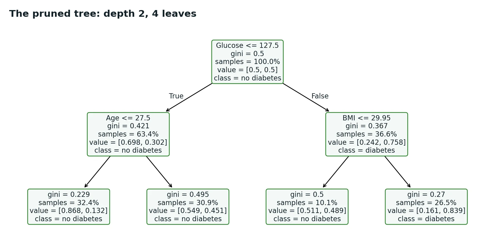
Four leaves. You could print it on an index card. Its test accuracy is exactly the same as the depth-5 tree's (75.3%), with 4 leaves instead of 26.
The catch: pruning quietly changed what the model is good at#
Here is the lesson I most want you to take away, because it is easy to miss. Same accuracy does not mean same model:
| Depth 5 | Depth 2 | |
|---|---|---|
| Test accuracy | 75.3% | 75.3% |
| Recall, diabetes | 0.815 | 0.556 |
| Recall, no diabetes | 0.720 | 0.860 |
The small tree catches only 56% of diabetic patients, down from 81%. It got its accuracy back by being right about healthy people instead. Both trees make 38 mistakes on the test set; they are just different mistakes. For a screening tool, the depth-2 tree is worse, even though a leaderboard sorted by accuracy would call them tied.
So "pick the depth with the best cross-validated accuracy" is only correct if accuracy is what you care about. For this problem you would tune for recall (scoring="recall") or F1 instead, and the answer might well change.
What to take away#
- A decision tree asks greedy yes/no questions, each chosen to reduce impurity the most.
- Look at your data before modelling: disguised missing values and class imbalance both change how you should read the results.
- Report cross-validated scores, not one lucky split.
- Deep trees memorise. Limit depth, leaf size, or both.
- Choose the metric from the real-world cost of each kind of mistake, then tune for that metric.
Would I deploy this model for medical decisions? No. At roughly 70% cross-validated accuracy, trained on 768 patients from one population, it is a teaching model. But as a way to understand the data, a shallow tree is hard to beat: in four leaves it tells you that glucose matters most, that BMI matters next, and roughly where the thresholds are.