

Imagine two groups of points on a sheet of paper and a ruler. Many straight lines separate them. Which one should you draw? A support vector machine (SVM) has a crisp answer: draw the line that leaves the widest possible street between the two groups, with the line down the middle of the street.
That one idea, maximise the margin, is why SVMs generalise well. A boundary that hugs one class too closely will misclassify the next slightly unusual point. A boundary with room on both sides has slack for the unknown.
In this article we build SVMs on a real diagnostic problem, and along the way meet the three things you must understand to use them: scaling, kernels, and the hyperparameters C and gamma.
The data: 30 measurements per tumour#
The Wisconsin breast cancer dataset ships with scikit-learn. Each of its 569 rows is a tumour, described by 30 measurements computed from a digitised image of a fine-needle biopsy: radius, texture, perimeter, area, smoothness, concavity and so on (each as a mean, a standard error, and a "worst" value). The label is malignant or benign.
from sklearn.datasets import load_breast_cancer
from sklearn.model_selection import train_test_split

bc = load_breast_cancer()
X_train, X_test, y_train, y_test = train_test_split(
    bc.data, bc.target, test_size=0.25, random_state=0, stratify=bc.target
)  # 426 training tumours, 143 test tumours
Why the street needs a common unit of measure#
Look at the ranges of just two of those 30 columns:
| Feature | Min | Max |
|---|---|---|
| mean area | 143.5 | 2,501 |
| mean fractal dimension | 0.050 | 0.097 |
An SVM measures distance between points. In raw units, a difference of 100 in area is a big number, while the entire range of fractal dimension is less than 0.05. So the distance, and therefore the margin, is decided almost entirely by the area-like columns. The fine-grained shape measurements might carry real diagnostic information, but the SVM cannot hear them over the noise of the big numbers.
The fix is StandardScaler, which rescales every feature to mean 0 and standard deviation 1. The pattern matters as much as the scaler:
from sklearn.preprocessing import StandardScaler

scaler = StandardScaler()
X_train_scaled = scaler.fit_transform(X_train)  # learn mean and std from TRAINING data only
X_test_scaled = scaler.transform(X_test)        # apply those same numbers to the test set
Fitting the scaler on the test set would let information about the test data leak into training. In practice the cleanest way to never get this wrong is a pipeline: make_pipeline(StandardScaler(), SVC()).
How much does scaling matter? I trained the same models with and without it:
| Kernel | Unscaled | Scaled |
|---|---|---|
| Linear | 94.4% | 96.5% |
| RBF | 91.6% | 95.8% |
The same algorithm, the same data, the same hyperparameters: two to four percentage points, from one line of preprocessing. For SVMs, k-nearest neighbours, PCA, k-means and anything else built on distances, scaling is not optional.
Support vectors: the points that matter#
After training the linear SVM, ask it how many support vectors it used:
from sklearn.svm import SVC

linear = SVC(kernel="linear", C=1).fit(X_train_scaled, y_train)
linear.n_support_   # [15, 14]
Only 29 of the 426 training tumours define the boundary. These are the points sitting on the edge of the street or inside it. Delete any of the other 397 and the model would not change at all. That is the "support vector" in the name, and it is why SVMs are memory-efficient at prediction time.
Kernels: bending the street#
A straight line is not always enough. The RBF (radial basis function) kernel lets the SVM draw curved boundaries. The trick behind it is elegant: it behaves as if the data were mapped into a much higher-dimensional space where a flat boundary works, without ever computing that mapping. All it needs is a similarity score between pairs of points, which drops off with distance.
On our tumours, with C=1 for both:
rbf = SVC(kernel="rbf", C=1, gamma="scale").fit(X_train_scaled, y_train)
# linear: 96.5% test accuracy,  RBF: 95.8%
The simpler linear model came out ahead. That is a useful result, not a disappointing one. Once the 30 measurements are standardised, malignant and benign tumours are largely separable by a flat boundary, and the extra flexibility of the RBF kernel has nothing to add.
But be careful how loudly you say it. The difference is one tumour out of 143. On 5-fold cross-validation over the whole dataset, the two are indistinguishable: 97.5% ± 1.0 for linear, 97.7% ± 0.7 for RBF. When a single test split gives you a one-sample difference, the honest conclusion is "tied".
C and gamma, visually#
The two knobs of an RBF SVM are easiest to understand on a toy dataset with two features, where we can draw the boundary. Below, the solid line is the decision boundary, the dashed lines are the edges of the margin, and circled points are support vectors:
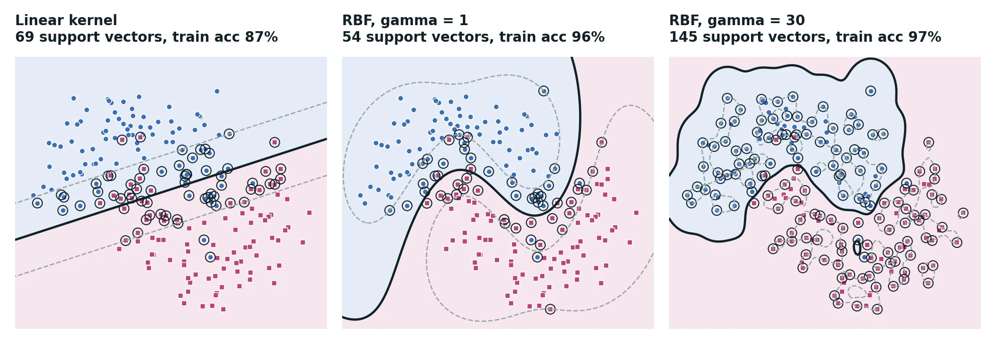
- Linear (left): a straight street through data that is clearly curved. 87% training accuracy; it underfits.
- RBF, gamma = 1 (middle): a smooth curve that follows the shape of the data. 96% training accuracy with just 54 support vectors.
- RBF, gamma = 30 (right): the boundary wraps around little islands of points. Training accuracy rises only to 97%, but now 145 of 200 points are support vectors. The model is memorising.
Gamma controls how far one training point's influence reaches. Small gamma: each point influences a wide neighbourhood, so boundaries are smooth. Large gamma: each point only influences its immediate surroundings, so the boundary can bend around individual points.
C controls how much the SVM cares about misclassified training points. Small C: allow some points on the wrong side in exchange for a wider street (more regularisation). Large C: insist on classifying the training set correctly, even if the street gets narrow and twisted.
When the number of support vectors climbs towards the size of the training set, that is a strong hint of overfitting.
Letting the grid decide#
Rather than guessing, search:
from sklearn.model_selection import GridSearchCV

param_grid = {"C": [0.1, 1, 10], "gamma": ["scale", 0.01, 0.1]}
grid = GridSearchCV(SVC(kernel="rbf"), param_grid, cv=5).fit(X_train_scaled, y_train)
grid.best_params_   # {'C': 1, 'gamma': 'scale'}
The winner is the default. gamma="scale" sets gamma to 1 / (number of features × variance of the data), which on standardised data with 30 features is 1/30 ≈ 0.033: a sensible middle value. The best cross-validated accuracy is 98.6%, and on the test set the tuned model scores 95.8%, the same as before tuning.
"Tuning found nothing better" is a real finding. scikit-learn's defaults are good for scaled data, and the grid confirmed it. Tuning earns its keep when your data is further from the defaults' assumptions, or when the grid is wider than nine combinations.
Mistakes worth reading#
On the test set, the linear SVM's confusion matrix is:
| Predicted malignant | Predicted benign | |
|---|---|---|
| Actually malignant (53) | 50 | 3 |
| Actually benign (90) | 2 | 88 |
Three malignant tumours were called benign. In a real diagnostic setting those three are the errors that matter most, far more than the two benign tumours sent for a second look. If this model were ever used as an aid, you would shift the decision threshold (via decision_function) to trade some false alarms for fewer missed cancers.
What to take away#
- An SVM finds the boundary with the widest margin; only the support vectors define it.
- Always scale features for SVMs, and fit the scaler on training data only. A pipeline makes this automatic.
- Try a linear kernel first. Reach for RBF when the boundary is genuinely curved.
- Gamma sets how local each point's influence is; C sets how much training errors are punished. High values of either push towards overfitting.
- A one-sample difference on one split is not a result. Cross-validate before you declare a winner.