

Every model so far in this series learned from examples with answers attached: this patient has diabetes, this review is positive. That is supervised learning. Unsupervised learning takes the answers away. You get the data and nothing else, and the job is to find structure that is really there.
Here is the setup. You are handed a chemical analysis of 178 wines, 13 measurements each: alcohol, malic acid, ash, magnesium, flavanoids, colour intensity, hue, proline and so on. Nobody tells you anything about where they came from. Do the wines fall into natural groups? How many?
The data does secretly come from three grape varieties (cultivars) grown in the same region of Italy. We will lock those labels away and only take them out at the very end, to score how well a label-free pipeline rediscovered them. They never touch a model.
from sklearn.datasets import load_wine

wine = load_wine()
X_raw, y_true = wine.data, wine.target   # y_true is ONLY for the final score
X_raw.shape   # (178, 13)
Step 1: the step that decides everything#
Look at how differently the 13 features vary:
| Feature | Standard deviation |
|---|---|
| proline | 314 |
| magnesium | 14.2 |
| colour intensity | 2.3 |
| hue | 0.23 |
| nonflavanoid phenols | 0.12 |
Both techniques we are about to use care about distances and variance. In raw units, proline varies thousands of times more than hue, so proline dominates everything. Run PCA on the raw data and the first component explains 99.8% of the variance, and that component is essentially proline alone. Twelve of the thirteen chemical measurements become invisible.
So we standardise first: every feature gets mean 0 and standard deviation 1.
from sklearn.preprocessing import StandardScaler

X = StandardScaler().fit_transform(X_raw)
We will measure exactly how much this matters at the end. (Spoiler: a lot.)
Step 2: PCA, or how much of this data is really there?#
Principal component analysis (PCA) finds new axes for the data. The first axis (principal component) points in the direction where the wines differ most. The second points in the direction of the next-most variation, at right angles to the first, and so on. Each component is a weighted mix of all 13 original features.
The useful question is how many components you need to keep most of the information:
import numpy as np
from sklearn.decomposition import PCA

pca = PCA().fit(X)
cumulative = np.cumsum(pca.explained_variance_ratio_)
k90 = int(np.argmax(cumulative >= 0.90) + 1)   # 8
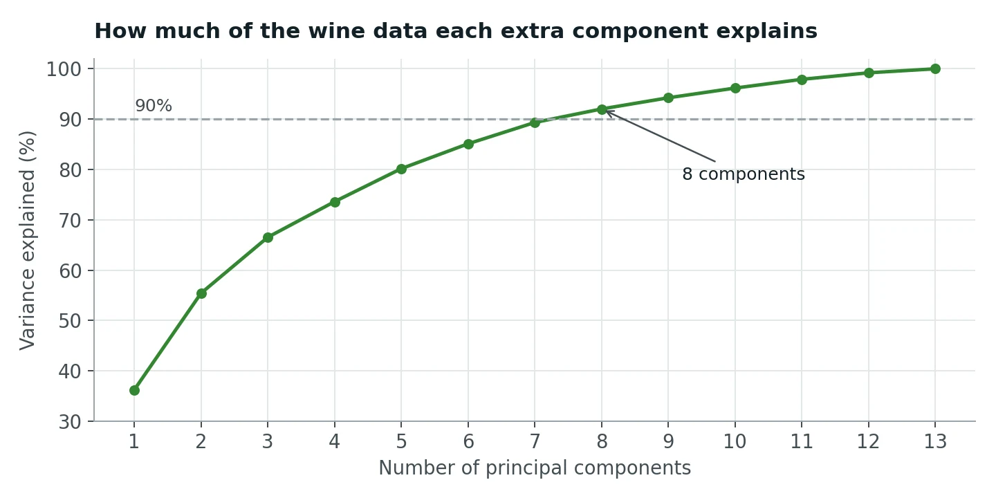
The first component alone explains 36% of the variation between wines, the first two together 55%, and it takes 8 components to pass 90%.
A common misreading is worth heading off: this does not mean 8 of the 13 measurements carry 90% of the information. Every component blends all 13 features. It means the variation in 13 dimensions can be summarised almost as well in 8 new dimensions, because many of the original measurements move together (flavanoids and total phenols, for example, are strongly correlated). PCA squeezes out that redundancy.
Step 3: k-means, and choosing k without cheating#
K-means is the simplest clustering algorithm there is. You choose k, the number of clusters. It places k centres, assigns every wine to its nearest centre, moves each centre to the average of its wines, and repeats until nothing changes. Because the starting positions are random, we run it 10 times (n_init=10) and keep the best.
But what should k be? We cannot peek at the labels. The standard label-free tool is the silhouette score. For each wine, it compares how close the wine is to the others in its own cluster with how close it is to the nearest other cluster. It ranges from −1 (probably in the wrong cluster) to +1 (tight and far from everything else), and we average it over all wines.
from sklearn.cluster import KMeans
from sklearn.metrics import silhouette_score

scores = {}
for k in range(2, 7):
    labels = KMeans(n_clusters=k, n_init=10, random_state=42).fit_predict(X)
    scores[k] = silhouette_score(X, labels)
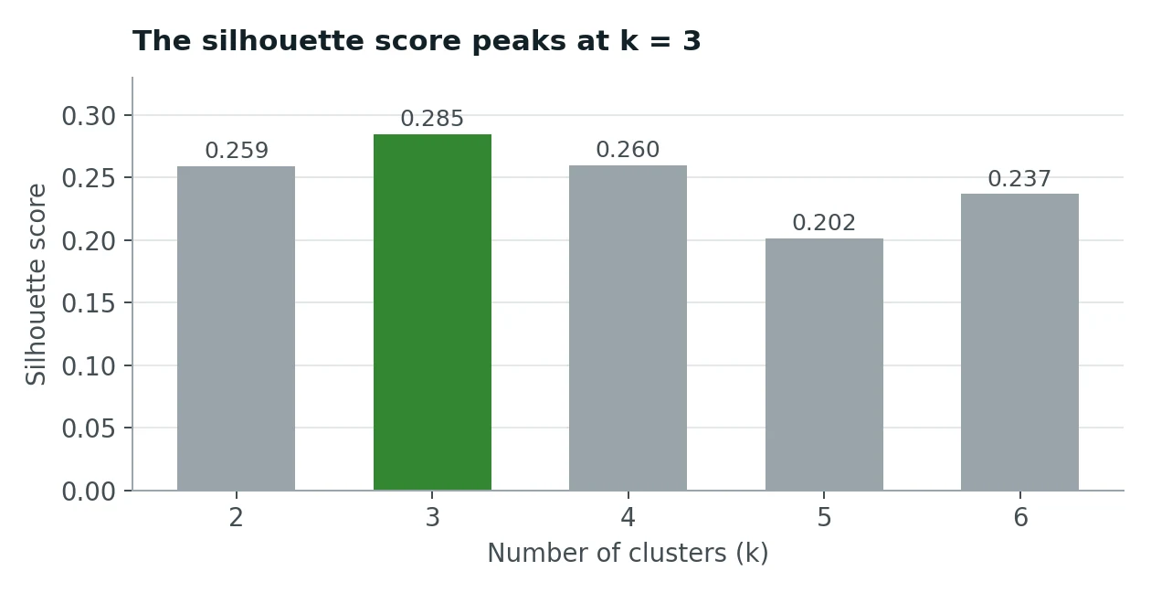
k = 3 wins with 0.285. Without ever seeing a label, the data itself suggests three groups.
Do not be alarmed that 0.285 looks low. Silhouette scores above 0.5 are rare on real data with 13 dimensions; what matters here is that k = 3 is clearly the best of the options. In a real project you would also look for a second, independent signal (an elbow in the k-means inertia curve, or stable clusters when you rerun on resampled data) before trusting a choice of k.
Step 4: now, and only now, open the envelope#
Time to compare the clusters with the true varieties. We cannot just count matches, because k-means numbers its clusters arbitrarily: its "cluster 0" might be variety 2. The Adjusted Rand Index (ARI) solves this by looking at pairs of wines: for every pair, do the clusters and the true labels agree on whether the two belong together? It is adjusted for chance, so random clustering scores about 0 and a perfect match scores 1.
from sklearn.metrics import adjusted_rand_score

clusters = KMeans(n_clusters=3, n_init=10, random_state=42).fit_predict(X)
adjusted_rand_score(y_true, clusters)   # 0.897
ARI = 0.897. Note that this is not "89.7% correct"; ARI is a pair-agreement score, not a percentage of wines. For the plain-English version, cross-tabulate:
| Cluster A | Cluster B | Cluster C | |
|---|---|---|---|
| Variety 1 (59 wines) | 59 | 0 | 0 |
| Variety 2 (71 wines) | 3 | 65 | 3 |
| Variety 3 (48 wines) | 0 | 0 | 48 |
172 of 178 wines (96.6%) landed in the cluster that matches their variety. Varieties 1 and 3 were recovered perfectly. The only confusion is 6 wines from variety 2, which sits chemically between the other two.
Seen in two dimensions (the first two principal components), the result looks like this:
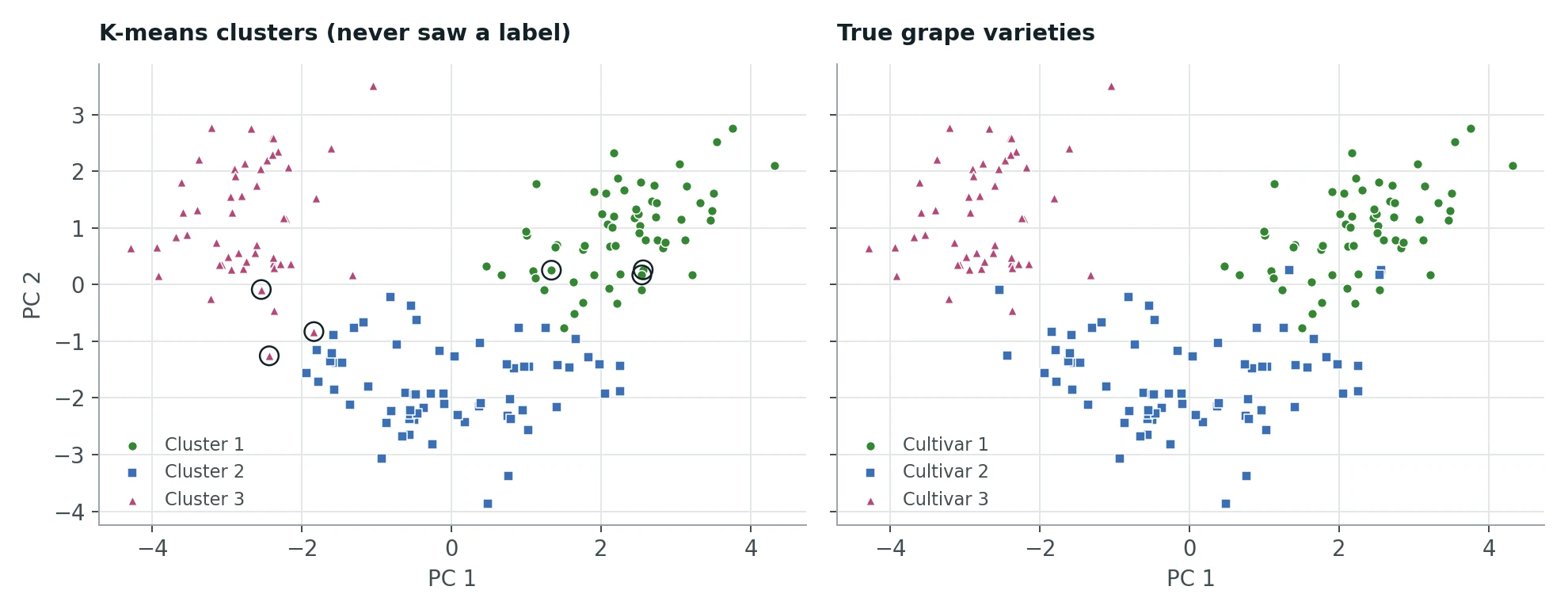
The left panel is what k-means found; the right is the truth. The six circled wines are the mismatches, all sitting on the borders between groups. Two dimensions show only 55% of the variation, so some separation you cannot see here does exist in the full data.
The scaling experiment#
Now the promised measurement. Run exactly the same k-means on the unscaled data:
| ARI | |
|---|---|
| Unscaled features | 0.371 |
| Standardised features | 0.897 |
Same algorithm, same k, same data. Without scaling, k-means is effectively clustering on proline alone, and proline by itself cannot separate the three varieties. One line of preprocessing is the difference between a mediocre result and an excellent one.
Two more small experiments: clustering on just the first 2 principal components gives ARI 0.895, and on the first 8 gives 0.897. So for clustering, PCA's main benefit here is speed and visualisation. Most of the useful structure already lives in the first two components.
When there is no answer key#
In a real project there is no y_true to check against. So what would convince you the clusters are real and useful? Two kinds of evidence:
- Internal: the structure is strong and stable. A clear silhouette peak at one k, agreement with other methods (hierarchical clustering, a Gaussian mixture), and clusters that barely change when you rerun on bootstrap resamples of the data. Structure that appears only with one random seed is not structure.
- External: the clusters mean something to someone. Profile each cluster (this one is high in proline and alcohol, that one high in malic acid and colour intensity) and show the profiles to a domain expert. Better still, check whether cluster membership predicts something you did not cluster on, such as price, region or customer rating.
What to take away#
- Unsupervised learning finds structure without labels; keep any labels you have strictly for evaluation.
- Standardise before PCA or k-means. Here it lifted ARI from 0.371 to 0.897.
- PCA components are blends of all the features. "8 components for 90% variance" is about redundancy, not about which features matter.
- Choose k with a label-free criterion such as the silhouette score, and confirm it another way.
- ARI measures agreement between groupings on a 0 to 1 scale. It is not a percentage of correct points; a cross-tabulation tells that story better.